The book published with the programs
|
|---|
|
The book was published in 1988. It included the source code (PASCAL) and notes about the programs |
|
|
|
|
|
|
| A simulation fitted to drawdown and recovery in an aquifer test |
There are many ways in which the programs might be used. Some examples are:
|
Home CG programs Index |
It should be stressed that these notes are concerned with using the CG set of programs for simulation and analysis of groundwater discharge test data. They are not designed, in themselves, as a course in hydrogeology, although it is hoped that they may provide a tool toward that end.
One of the available consistent sets of units is recommended for analysis.
The well test data recorded on disk is independent of the set of units that you choose. The set of units is recorded as a part of the current configuration.
|
Home Top Index |
You will come back to the primary menu after all the major operations; data entry, graphing, simulation, analysis, etc. As soon as you select one of these options from the primary menu, CG will call up an autonomous program and also will pass some information to that program.
As you use the CG programs you will see several menus which look very like the primary one. There are two ways of selecting an option from these menus: you may use the up or down arrow keys to move the highlighted bar to the option and then press [Enter], or you can press the 'hot key' (the numeral or letter key on the left margin). (Pressing the up arrow when at the top of the menu will get you to the bottom, and vice-versa.)
I suggest that you use the former method as you are getting to know the programs because you will be given a short explanation of each option as you scroll up or down the menu.
Most of the other programs can then be used to examine or analyse this data file in one way or another. Some methods of analysis look at the whole data set, others look only at some aspect of the data, yet others look at several data sets simultaneously.
The sole purpose of two programs is to produce simulated data. These are written to files in the same way as the field data that you enter. The simulations can be very useful for comparison with field data and also for educational purposes.
Inclusion of well storage effects is an option in the production of simulated well test data and compensation for well storage effects is an option in the analysis of well test data. However, these programs do not make any allowance for well storage effects in the simulation or analysis of aquifer test data.
|
Home Top Index |
This file will contain a table of values derived from the well equation that you have evaluated for a particular well (refer to the Well Equation below). All the data in the file will relate to a single duration of pumping that you specify when you create the file.
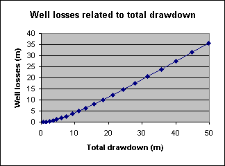
The first column of the file will contain a series of 20 discharge rate values. The second column will contain drawdown values for the corresponding discharge rate. The third column will contain specific capacity (Q/s) values. The remaining three columns will contain the value of the A term, B term, and C term of the well equation, again for the corresponding discharge rate. Each column will be separated by a comma so that the file may conveniently be 'imported' into a spreadsheet. (The commas are automatically recognised as deviders so that each value goes into a different column.)
An example file is given in table 1...
Q,s,Q/s,A term,B term,C term
100.000000,0.72000000,138.888889,0.70000000,0.0,0.02000000
200.000000,1.51313708,132.175731,1.40000000,0.0,0.11313708
300.000000,2.41176915,124.390015,2.10000000,0.0,0.31176915
400.000000,3.44000000,116.279070,2.80000000,0.0,0.64000000
500.000000,4.61803399,108.271182,3.50000000,0.0,1.11803399
600.000000,5.96363261,100.609819,4.20000000,0.0,1.76363261
700.000000,7.49283628,93.4225670,4.90000000,0.0,2.59283628
800.000000,9.22038672,86.7642567,5.60000000,0.0,3.62038672
900.000000,11.1600000,80.6451613,6.30000000,0.0,4.86000000
1000.00000,13.3245553,75.0494089,7.00000000,0.0,6.32455532
1100.00000,15.7262320,69.9468252,7.70000000,0.0,8.02623199
1200.00000,18.3766127,65.3003915,8.40000000,0.0,9.97661265
1300.00000,21.2867633,61.0708157,9.10000000,0.0,12.1867633
1400.00000,24.4672970,57.2192344,9.80000000,0.0,14.6672970
1500.00000,27.9284251,53.7087214,10.5000000,0.0,17.4284251
1600.00000,31.6800000,50.5050505,11.2000000,0.0,20.4800000
1700.00000,35.7315505,47.5770006,11.9000000,0.0,23.8315505
1800.00000,40.0923117,44.8963885,12.6000000,0.0,27.4923117
1900.00000,44.7712504,42.4379481,13.3000000,0.0,31.4712504
2000.00000,49.7770876,40.1791285,14.0000000,0.0,35.7770876
|
| Figure 1. Well losses related to total drawdown (data from the table above) |
The graphing of selected columns taken from a file such as this can provide useful insights into the functioning of the well.
|
Home Top Index |
The naming of the well characteristics file is automatic. The file name has the form 'WCHnnn.csv' where nnn represents a three figure number. The file name extension, 'csv' indicates that the file is written in comma delimited ASCII (the American Standard Code for Information Interchange) format. If there are no files with names matching WCHnnn.csv in the current data directory then if you create a file it will be named WCH001.csv. If WCH001.csv already exists then the new file will be WCH002.csv, etc., up to WCH999.csv.
When you are analysing data from the data files it will be obvious that each plot on a graph must have a time value and a drawdown value. Much less obvious, but of great importance, is the fact that each point also has a discharge rate value. It is this that allows the CG programs to take into proper consideration the periods of recovery or of differing discharge rate.
Examine several files using CGEdit to familiarise yourself with their forms. A file that contains stepped rate data from a well test might be most instructive, try WOOL38B.
From the primary menu select CGEdit (Data entry and editing). You will be asked if you want to load a data file, reply with [Y]. You will now be given a file name and asked if you want to load it, if it is not WOOL38B then reply with [N]. Now select WOOL38B from the list displayed, using the arrow keys and then pressing [Enter].
Now display the data by selecting Data entry/editing from the CGEdit menu. You can scroll through the data using the [PgDn] and [PgUp] keys.
Data files will be read from, and written to, the 'current data directory'. After you install the programs you must change the current data directory to match the name of the directory you want to store data in and retreive data from.
To change the current data directory select 'Change configuration' from the primary menu and then select 'Change path'. The program will give you a list of the subdirectories attached to the directory containing the CG programs. Type in a valid data file directory name if you wish to change it, otherwise press [Esc] to retain the existing name.
If you want to create a new subdirectory for well test data files then you will need to exit from the CG programs and use Windows Explorer to create a new directory.
|
Home Top Index |
In every case a notes file will be written, in addition to the data file, to record information on the particular simulation. The notes file will have the same name as the data file except that while the extension part of the data file name will be '.CTD' that of the notes file will be '.CTN'.
The data will be written to a file having a name in the form SIMnnn.CTD, where 'nnn' represents a three digit number. The system can best be explained by example. If there are no files of this type in the currently selected data directory and you cause a file to be written, it will be named SIM001.CTD. If file SIM001.CTD exists then the data will be written to file SIM002.CTD etc. The maximum is SIM999.
The command to write the file is given by pressing [F] (for 'file') whenever you are using the Manual generalised method and there is a simulation on the VDU screen.
Simulations produced by CGAnal and CGPAnal will have identical times and discharge rates to those of the measured data files.
The simulation will be written to disk whenever you press [F] while the simulation is on the screen.
A text search is also available from the Help menu, press [S] and type in the text that you are interested in. Pressing [A] will then find the next occurrence of the same text.
|
Home Top Index |
A short explanation is given in parentheses where it seems to be warranted. Remember that more information is given from the menus and from the help system. Table 2
DATA EDITING, MAIN MENUAquifer test simulation
Data entry/editing
Special editing
DATA EDITING MENU Right (move cursor to next field right) Left (move cursor to next field left) Next record (move cursor to next record) Previous record (move cursor to previous record) Back up 16 records (move cursor back 16 records) Forward 16 records (move cursor on 16 records) Edit this field (edit the field under the cursor) Add new data to end (append data to the end of the file) Add constant (add a numeric constant to one or more numbers in the current column) Multiply by constant (as above, but multiply) Insert one record (insert at cursor's position) Delete record(s) (Delete one or more records from cursor's position toward end of file) Back to main menu (Exit to next higher menu) SPECIAL EDITING MENU
Simulate full recovery (For step test data) Randomise drawdowns (Add a 'field' error to simulated data) Simulate confined Simulate unconfined Correct for background (Correct for changes observed in a piezometer monitoring background noise) Change test description (Well diameters, etc.) Merge with file (Join current data with file data) Sort (into chronological order) Correct for residual (Correct for preceding pumping) Return to main menu
CG ANALYSIS MENU
Transmissivity
Storage coefficient
Leakage coefficient
Theisfit
Leakyfit
Automatic generalised
Manual generalised
Slug test
Change maximums (Change the limits on the graph)
End
|
Home Top Index |
HOT KEYSMultiple well fit
Modification of A, B, C, D, t, Q, Un/confined, Isotropic/strip
Output of s vs. Q and Q/s vs. Q in delimited file
INDEX MENUChange configuration
Browse or edit
BROWSE EDIT MENUChange field names
Previous record
Next record
Insert a record
Delete a record
Exit
Change field (Replace contents of field) Find in priority field (Refer to notes on index, below) Search in any field (Refer to notes on index, below)
Change sort order
Exit
CG CONFIGURATION MENUExit to DOS
Customise colours
Change path (Change the DOS path for data files) Units (Select different units)
Exit
You can write in the notes files via the main menu of program CGEdit; or you can, if you prefer, use an ASCII editor program. The only rules about how the notes files should be formatted are that the lines must not be longer than 76 characters and there must be no more than 18 lines in a file. If you are using CGEdit to write your notes files you need not worry about these rules, CGEdit will keep you within the limits. When you exit from viewing and/or editing the notes file you have the option of writing it, with any modifications that you might have made, to disk.
CGEdit also provides a scan feature. With this you can quickly scan through the notes files in a given directory. You cannot modify the notes files from the scan mode.
|
Home Top Index |
The discharge test simulation programs will produce notes files whenever they write a simulation to disk. The note file will record the specifications that you used when you produced the simulation.
The help system will give you more information on the notes files.
The index is kept sorted. It can be sorted on any field, the sort specification is up to you; you will probably use different specifications for different purposes. You might be looking for file relating to a certain project at one time, or files from tests carried out on a particular date at another time.
The index is in capital (upper case) letters. You may enter data in either upper or lower case, but everything will be converted to upper case.
Note that this is a simple index. If you want something more powerful and elaborate you will probably be well advised to use a data base manager.
Two items in the Browse/edit menu of the file index system should have a little explanation.
Particularly if the analysis that you are working on is an important one and your report is going to result in commitments being made involving major expenses, then you should very carefully check your results.
As stated elsewhere, most of the data handling and analysis operations are done using the consistent set of units based on metres and days. If your analysis was done in other units then one check that you could do is to change to the metre/day set and repeat the analysis, checking that the results are the same.
You should not rely entirely on the CG programs, run an independent check by some other method if the results are important.
If you should find any errors, then please inform me of them, so that I can correct them.
|
Home Top Index |
Whatever your preference for the time unit used in analysis, you are free to enter field data in any units at all; you can change units after you have completed data entry (for that matter you can change time unit half-way through data entry if you like).
Suppose your reading times were something like the following: 30 seconds, 1 minute 20 seconds, . . ., 55 minutes, 1 hour, 1 hour 10 minutes, . . ., 26 hours, 28 hours, etc.
The easiest way to enter these times would be to start data entry using minutes, and change the time unit to hours after entering the 55 minute reading. You would enter the seconds as sexagesimal fractions, eg. 30 seconds would be entered as 0;30, 1 minute 20 seconds as 1;20. After switching to hours you would similarly enter 1 hour 10 minutes as 1;10.
Throughout this you could be entering discharge rates in cubic metres per day, litres per second, US gallons per hour, or one of several other units.
The time-drawdown curve, when plotted as a semilogarithmic graph, shows a straight line following an initial downward curve.
At early times the drawdown curve is identical to that of the Theis curve, but at later times drawdowns become progressively less, finishing in a horizontal line if discharge continues for a sufficient period.
The equation is: (apology, html is not great for writing equations)
| Equation 1 |
| Sc = Su- | Su2 2D |
The inverse of the Cooper-Jacob equation will convert drawdowns
measured in (or simulated for) a confined aquifer to approximate values
which would be expected in an unconfined aquifer having similar characteristics. The inverse of the Cooper-Jacob correction is:-
|
Home Top Index |
| Equation 2 |
| Su = D(1-root(1- | 2Sc D | ) |
|
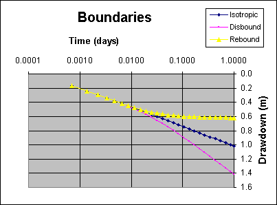
| Figure 2. Effect of a discharge boundary and a recharge boundary |
There are two primary types of boundaries, discharge and recharge. The discharge boundary is a line through which no water may pass. It corresponds to the edge of the aquifer or an impermeable dyke, etc. The recharge boundary is a line source of unlimited water, such as a stream which fully penetrates the aquifer.
On a semilogarithmic graph the effect of a discharge boundary is to double the slope of what otherwise would be the straight line section of the curve. The recharge boundary results in the curve becoming a horizontal line for later times, as the point is reached where all the water flowing to the well is coming from the boundary.
Figure 2 shows a comparison of (upper curve) recharge boundary, (middle curve) no boundary, and (lower curve) discharge boundary. The middle curve is the data of example file CONF0030, while the other data for the other two curves were produced by the 'Manual generalised solution' of the aquifer test analysis program (CGAnal). The values used for CONF0030 were: T=200 m2/day, S=0.0001, R=30 m, Q=300 m3/day for 1 day. The discharge boundary model included a discharging image well at a distance of 400 metres from the piezometer, while the recharge boundary model had a recharging image well at the same distance.
|
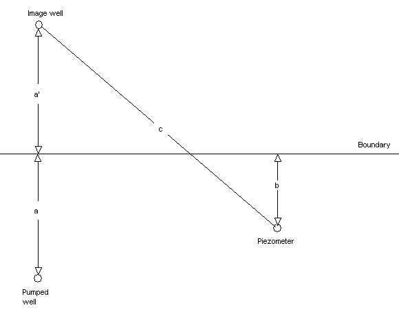
| Figure 3. Single boundary, distances |
When you specify an aquifer configuration containing a boundary the programs will ask for the distances that are needed to define the model.
|
Home Top Index |
As illustrated in the Figure 3, the distance from the pumped well to the boundary (a) is equal to the distance from the boundary to the image well (a').
Figure 4 is a simulation showing the effects of a partial boundary on drawdown in a confined aquifer. Here, the upper curve is the case where there is no boundary, the lower curve is a full discharge boundary, while the middle curve is a partial boundary where the transmissivity on the side of the aquifer containing the wells has been taken to be twice that on the far side of the boundary. The Delta s slope for the partial boundary is approximately half way between those of the unbounded and fully bounded cases. (Delta s is defined as the drawdown per log [base 10] cycle.)
|
| Figure 4. Effect of a 'partial' boundary |
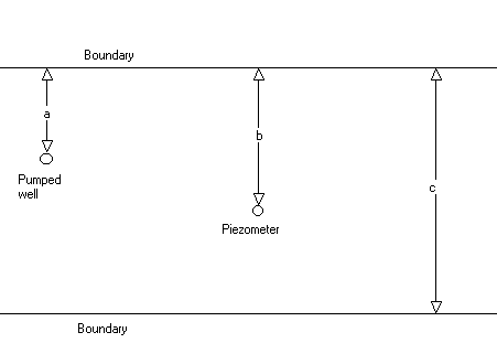
The strip aquifer case requires the same three distances needed in the single boundary case and also the width of the aquifer, c in Figure 5.
In this case there are, of course, an infinite number of image wells.
The image wells are created by 'reflections' of the pumped well, with
the boundaries acting like mirrors. The program considers image wells
further and further from the piezometer until the point is reached
where their effect is negligible.
|
| Figure 5. Strip aquifer, distances |
|
Home Top Index |
As is the case in manual analysis of discharge test data, many of the methods provided here are applicable only to data from discharge tests where the discharge rate was held constant.
In general the aquifer analysis methods deal with data from piezometers while well analysis deals with data from the pumped well. There are many exceptions to this, however, eg. slug analysis is an aquifer test which uses data from the pumped well, and transmissivity can be derived from a multistage well test.
Two methods available in the aquifer analysis program, CGAnal, are capable of considering data from tests which include variations in discharge rate. These methods, the 'automatic' and 'manual generalised' methods, therefore can take into account recovery data. I strongly suggest that recovery data should be included when these methods are used, as it provides something of an extra perspective on aquifer performance.
Most other methods are applicable to data containing changes in discharge rate so long as they are used on the part of the data before the change occurred.
This method is used by the aquifer test analysis program, CGAnal. The calculation of Delta s will be independent of the type of graph being used to display the data.
Transmissivity is calculated from Delta s by the equation:
| Equation 3 |
| T = | 0.183 Q ______ Delta s |
| Equation 4 |
| T = | 0.183 _____ B |
The best fit Theis type curve is found for the specified section of the data. Changes in discharge rate before or during the chosen section are not allowed.
The best fit leaky-artesian (Hantush, 1955) type curve is found for the selected subset of the data. Changes in discharge rate are not permitted before or during the selected data. This solution will fail to converge in many cases where there is not a close match to a theoretical type curve.
|
Home Top Index |
Five methods are available in the aquifer test analysis program (CGAnal), and another from the 'Multiwell fit' accessible from the primary menu.
The storage coefficient (or specific storage or storativity) is evaluated by solving the two equations below for S.
| Equation 5 |
| u = | root(R) S _______ 4 T t |
| Equation 6 |
| S = | Q W(u) ______ 4 pi t |
Of the above, only T, and S itself are unknown. You will be requested to enter the value of T and then S will be evaluated.
(The well function of u is evaluated using a polynomial approximation detailed in Clarke 1988. The solution of the above equations for S, by Newton's method, is described in the same publication.)
|
Home Top Index |
Note that the assumption is made that the aquifer is a simple confined isotropic one. If this is not justified, eg. the effects of a boundary or leakage are apparent at the time of the selected drawdown figure, then the derived figure for S will be in error. I suggest that the point selected for use in the evaluation be carefully considered bearing this in mind.
It may be useful to provide some equations relating these values to each other. (I have given more equations than are really needed. In my experience hydrogeologists are not always dazzling mathematicians. {Just as programmers are not always brilliant spellers!})
|
Home Top Index |
| Equation 7 |
| L = root( | T b ___ K' | ) |
| Equation 8 |
| c = | L2 __ T |
| Equation 9 |
| c = | b __ K' |
On the assumption that the Cooper-Jacob approximation gives a good characterisation of unconfined drawdown it is theoretically possible to evaluate the aquifer thickness from the time-drawdown curve (using either the automatic or manual generalised methods of CGAnal). In practice I would expect that unknown and extraneous factors would be too great to make this a practicality.
It should be remembered that the derived image well distance is going to be dependent on the uncertainties in T and S, and that these are usually substantial.
|
Home Top Index |
The user defines the aquifer model and then enters first guesses for the aquifer parameters. The solution then systematically searches for changes that can be made to the parameter values which will lead to a reduced root-mean-square error. It starts by attempting large changes and progressively moves toward smaller changes, finally, when all factors have been reduced to below 1.02 the procedure terminates. The factors for adjusting the parameter values start at two and are progressively reduced by replacing the old values with their square roots.
An example of the use of the Automatic generalised solution is given in the tutorials.
Several examples of the use of the Manual generalised solution are given in the tutorials.
Also see the comments on strip aquifer analysis under the 'Automatic generalised solution' above.
|
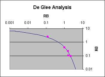
|
Best fit DeGlee analysis for well Waik6. T=27m2/day,
L=334m.
A modification to the CG Programs (2003/06/07) allows a data dump to a .csv file suitable for convenient importation into a spreadsheet. To dump, press S or L with the graph on the screen. The data will be written to a file named Deglee.csv. |
There are two options for data entry, either the data are entered via the keyboard, or the program reads the data from the discharge test data files. Note that the assumption is made that drawdown in the piezometers has reached steady state.
The method operates by first plotting the Hankle function (the Bessel function of the second kind and zero order). The next step is to plot R/Ro against s/so for each piezometer. (Where R is the distance between the particular piezometer and the pumped well, s is the steady state drawdown in the particular piezometer, and Ro and so are constants.)
Ro and so are now adjusted to produce the best possible fit between the data and the plotted Hankle function. This is first done automatically then the fine adjustment is performed manually.
Transmissivity is calculated from the equation:
| Equation 10 |
| T = | Q ____ 2 pi s0 |
|
Home Top Index |
There is a tutorial on the use of the DeGlee analysis below.
In my opinion a slug test may be useful in getting a quick approximation of hydraulic conductivity/transmissivity, but is no substitute for a full discharge test.
Well test analysis deals only with time-drawdown-discharge rate data from the pumped well.
The primary well equation, as used here is:
| Equation 11 |
| s = AQ + BQ log(t) + CQD |
|
Home Top Index |
These two forms of the well equation assume negligible storage within the pumped well. A correction for well storage effects is available in both the simulation (CGPDD) and analysis (CGPAnal) programs. The correction uses the figure that you provide for the radius of the well in the area where the water level is rising and falling to calculate the well storage. It is an iterative method which seems to give a good simulation of reality.
When you use the well test analysis program (CGPAnal) you will be asked whether you want a preliminary analysis, in most cases you will reply yes to this as it will normally provide a good first approximation faster than can be achieved manually.
If you decide not to use the preliminary analysis then you will be asked for initial estimates for the four coefficients, A, B, C, and D. The numbers that you give will depend greatly on the set of units that you are using. When proficiency with the program is gained you will be able to find a quick solution even when your initial estimates were very far from the mark, but at the learning stage this may cause difficulties.
Typical initial values are:
| Units | A | B | C |
| Metres/days | 0.01 | 0.001 | 10e-6 |
| Metres/seconds | 500 | 100 | 10000 |
| Feet/days | 0.001 | 10e-4 | 10e-8 |
| Feet/seconds | 30 | 10 | 70 |
The best approach in using CGPAnal is to first evaluate coefficient B, as all the other coefficients are, to some extent, interdependent. (To begin adjusting B, press [2].) If your data include a recovery period then I suggest that you evaluate B from that, if there is no recovery period then evaluate B from the slope of the first stage (see also the notes on evaluation of transmissivity).
Next, progressively evaluate coefficients A and C. Adjust A to obtain a good fit for the stage having the lowest discharge rate, then adjust C to produce a good fit for the stage having the highest discharge rate. Repeat this process until the fit is sufficient for your needs (probably two or three times).
If your test consists of at least three stages and the fit with the intermediate stages is not good enough you can adjust coefficient D (the exponent in the third term). An increased exponent will produce proportionally greater drawdown at higher discharge rates than at intermediate rates. (Coefficient C will automatically be adjusted as you change D, but you will need to modify both A and C to optimise the simulation.)
The CG programs can provide a dynamic and very interactive educational resource to help students visualise how time/drawdown type curves change according to the aquifer characteristics.
|
Home Top Index |
Back at the primary menu pick CGPlot (Data plotting). You will be asked if you want to load some specified file. The specified file will be the one that has most recently been written to, or read from disk. For this exercise you need file 'CONF0100'.
(The full file name is 'CONF0100.CTD' but you just need to concern yourself with the first part of the name, the CG programs will add the second part. The file contains data simulated for a discharge rate of 300 m3/day, a duration of one day, a transmissivity of 200 m2/day, a storage coefficient of 0.0001, and a piezometer 100 metres from the discharging well.)
If the given file name is not CONF0100 then answering with [N] will cause a list of data file names to be displayed, and among those will be the one you want. Use the arrow keys to highlight CONF0100 and then press [Enter] to load this file into memory.
This data file is simulated time/drawdown/discharge rate data for a simple confined (Theis) aquifer. (The standard assumptions have been made, the aquifer is presumed to be infinite in extent, isotropic, fully confined, and the well is considered to have no storage; ie. to have an infinitesimal radius. Unrealistic, but quite good enough for a great many real situations.) Ask CGPlot to provide a screen graph.
The first graph will be linear, the simplest of them all. Select this by pressing [L]. Answer [N] to 'Alter any drawdown or time limits', and either [Y] or [N] to 'Join data points'. Notice that the water level in the piezometer fell very quickly in the early stages of discharge, and progressively more slowly at later times. Also notice that while the rate of fall declined, the fall did continue until the end of the simulation; in theory it would continue for ever.
Pressing any key (except [S] or [L]) will clear the graph from the screen and cause the question 'Exit or Another graph?' to be displayed, answer with [A]. Tell CGPlot that you do want to load CONF0100. The next graph we will view will be double logarithmic, that is, one having logarithmic time and drawdown scales on the axes. Pick this by pressing [O]. The data of file CONF0100 will now be displayed as a log-log graph. This is the form of graph traditionally used for type-curve matching. You will notice that time increases from left to right and drawdown increases from bottom to top.
Next, after exiting from the log-log graph and reloading CONF0100, select a semilogarithmic graph. While the time scale is exactly the same as for the previous graph, this time the drawdown scale is linear; it also increases from top to bottom, more reminiscent of a falling water level in a piezometer. Perhaps the most important point to notice, however, is that after a short curved section all the data points fall on a straight line. This straight line can be used to calculate the transmissivity of the aquifer (the operation is described elsewhere).
|
Home Top Index |
The last type of graph that you should have a quick look at here is the root time graph. With this data it has some resemblance to the linear graph, but you will notice that the scale along the x axis is not linear, and the early time data are not so crowded up on the left. This type of graph is useful in examining data from a strip aquifer, when the later time data points will fall on a straight line (described elsewhere).
A discharge boundary is a line beyond which the aquifer does not exist. It might be something like a granite 'wall' at the edge of an alluvial gravel aquifer in a valley bottom. It is called discharge because its effect is identical to that of a discharging image well.
A recharge boundary is a line where no decline in the piezometric surface can be produced, no matter how much water is withdrawn from the aquifer. An example is a river fully penetrating the aquifer. It is called recharge because its effect is identical to a recharging image well.
Two example data files are provided: DISBOUND simulates the effects of a discharge boundary while REBOUND simulates the effects of a recharge boundary. Both can be compared with CONF0030, where the aquifer characteristics are taken to be the same apart from the boundary. In both cases the boundary is 200 metres from the piezometer and the same distance from the discharging well.
If you have changed the units then bring them back to the consistent set based on metres and days, as described in Tutorial E1. File CONF0030 is an identical simulation to file CONF0100 of Tutorial E1 except that the piezometer is now 30 metres from the discharging well.
From the primary menu choose CGPlot (Data plotting) and load the three files CONF0030, DISBOUND, and REBOUND; and then display them on a similogarithmic graph. You will notice that the curve of CONF0030 is very much the same as that of CONF0100 (of Tutorial E1) while DISBOUND falls away below and REBOUND rises above. What is not so obvious is that the slope of the DISBOUND curve approaches exactly twice that of CONF0030 while that of REBOUND approaches zero (a horizontal line). (This is reasonable on consideration of the image well model; in the discharge boundary case the extraction is doubled so the slope is also doubled, in the recharge case the total extraction is zero, so the slope approaches zero.)
|
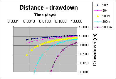
| Figure 6. Distance/time/drawdown |
To simultaneously view all of these files select CGPlot (Data plotting) from the primary menu. Answer [N] to the question 'Do you want to load file xxx alone' and then select the five files shown above by using the arrow keys and [Enter]. Press [F10] when all five file names are highlighted.
|
Home Top Index |
All of these data files were produced by CGDD, the aquifer test simulation program. Note that the 'piezometer' at 10 metres (file CONF0010, the upper curve) already has 0.4 metres drawdown at one minutes discharge. In practice this would, in most cases, be obscured by well storage effects in the pumped well and in the piezometer.
You can produce your own simulations along similar lines if you wish. Of course you are not restricted to a simple confined aquifer, you can add a boundary, leakage, strip aquifer effects, changes in discharge rates, periods of recovery, etc.
From the primary menu select CGAnal (Aquifer test analysis), load file CONF0100, and select a double logarithmic graph by pressing [O]. From the CGAnal menu select the Manual Generalised solution, specify a confined aquifer with no boundaries. Indicate that no aquifer parameters are known. As your 'first guesses' give T=200 m2/day and S=0.0001, exactly as used to produce the simulation.
A graph will now be displayed, it will show the data from the file, and over that the simulation produced according to your specifications. As the two will exactly coincide you will see only one set of data.
At this point we can change the value of transmissivity (T) for the simulation by pressing the up or down arrow keys, but before you do that press [C] then press the up arrow key until the number displayed as the 'Current adjustment' is about 2.14, then press [C] again.
The 'current adjustment' is the factor used to multiply by T every time you press the up arrow. It was set at a small number so that a user could adjust it to fit a type curve to file data, but that is not our present purpose. Now a press of the up or down arrow keys will change T by roughly a factor of 2. Try modifying T, then bring it back to its original value.
To switch to adjusting storage coefficient (S) press [2]. ([1] selects T, [2] selects S.) Again, before changing S press [C] and change the 'current adjustment' as you did for T. Now you can modify either or both T and S and observe the effect on the type curve.
Call up CGAnal, but load file LEAKY instead of CONF0100. (LEAKY is a simulation based on the same values as file CONF0030 with the addition of a leakage coefficient of 500.) Call the 'Manual generalised' solution as before, and give T=200, S=0.0001, and L=500. Now modify T, S, and L in a similar way to Tutorial E4. You might find it best to use a smaller adjustment for L than 2, as the effect of leakage is proportional to the square of the value of L. You will notice that increasing L decreases the amount of the actual leakage.
|
Home Top Index |
When the graph is on the screen, press 3 to select image well distance as the current parameter. Now use the up and down arrow keys to modify the image well distance and note the effect on the curve. You may like to increase the magnitude of the factor used to modify the image well distance, to increase the size of the changes.
You will find that increasing the image well distance moves the curved section of the graph to the right, toward greater times; while decreasing it has the opposite effect.
You might like to repeat this exercise with file ReBound (recharge boundary).
|
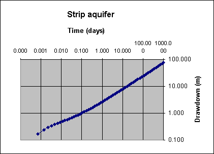
| Figure 7. Strip aquifer response - straight line on log-log graph |
Exit from this graph and plot all three files on a square root of time graph. This time you will see that while CONF0030 and DISBOUND both curve upward, the later data points of STRIP fall on a straight line, the most useful feature of the root-time graph.
The later time points of strip aquifer data plotted on a log-log graph also fall on a straight line, but this simulation is not really long enough to demonstrate that; however, the same simulation carried on to 1000 days does demonstrate it very effectively, as shown in Figure 7. (The scale of the drawdown in Figure 7 is not very realistic, but the point is made.)
From the beginning of discharge the cone of drawdown moves out in a circle around the pumped well. It ceases to be circular when it intercepts one or more boundaries. As the cone intercepts boundaries so it steepens inside the strip. The time at which boundary effects will start to show up will depend on the distances between the pumped well and the nearest boundary, and the piezometer and boundary. More precisely, it will depend on the distance between the piezometer and the closest image well (see the notes on bounded and strip aquifers above).
|
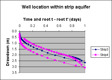
| Figure 8: Effect of well location within a strip aquifer |
Also note in Figure 8 that the recovery data from the simulations (the upper, shorter lines), at least when plotted as the square of root t minus root t', quickly become indistinguishable from each other.
|
Home Top Index |
|
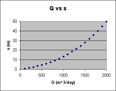
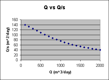
| Figure 9. Discharge rate versus drawdown |
To produce a simulated well test data file, run CGPDD (the pumped well simulation program). Request an isotropic confined aquifer and give values of A=0.007, B=0.0016, C=2e-7, and D=2.5. The discharge rates and durations should be Q=500, 800, and 1300 against t=100, 200, and 300, respectively. Give 0.1 metres for both well radii, and save the output to disk. Call CGWellEq (Well equation) from the primary menu. Accept the values given as they will be the same as those you used in your simulation and press [F]. Give 30 minutes as the time for the calculation of drawdowns and 2000 cubic metres per day as the maximum discharge rate. The data will now be written to a file called WCHnnn.ASC, in the current data directory (directory CGXample, unless you have changed it).
Refer to the notes on 'Well characteristics files' for information on the structure of the file that you have created, and for more information about its name.
Figure 9 shows discharge rate plotted against drawdown, and Figure
10 shows discharge rate plotted against specific capacity; both
being produced from the output produced by this exercise.
|
| Figure 10. Discharge rate versus specific capacity |
Please do not just follow these instructions to the letter, it is by experimentation that you will best learn the strengths, and the limitations, of the CG programs.
|
Home Top Index |
If you have not already done so, start the CG programs by changing into the correct directory, typing 'CG', and pressing [Enter].
While still at the primary menu, select 'Change configuration' and then 'Units'. Make sure that the units are the consistent set based on metres and days. They should be: metres, days, m3/day, m2/day, and m/day, and there should be a statement to the effect that they are consistent. If not please change them until they are. Leave the 'Units' area, but do not leave the Configuration menu yet.
The file that contains the data for this tutorial is in the subdirectory 'CGXAMPLE'. Select 'Change Path' and, if necessary, change the path to 'CGXAMPLE'; this only involves typing in the word and pressing [Enter]. Once the path is set at CGXAMPLE and has been accepted, leave the 'Change path' area and also leave the 'Configuration' area.
From the primary menu select 'Aquifer test analysis'. You will be asked whether you want to load a file. If the file name given is 'CONF0030' then answer [Y] for yes, otherwise answer with [N] and then select CONF0030 from the list that you are shown.
Next you should choose a semilogarithmic graph. (This graph is chosen in this case because the later time data will always fall on a straight line on this type of graph, given a confined aquifer and a sufficiently long and steady discharge rate.) You will now be shown some information on the data file, unimportant in this case; pressing any key will get you to the main menu of this program (named CGAnal).
For the first step we will make an estimate of the transmissivity, so choose transmissivity from the menu. You will be asked to set a marker at the right end. This marker will indicate the last reading to consider in the analysis; you should, in this case, set it right at the end of the graph by pressing the right arrow several times, then press [Enter] to anchor it. Notice that while you are moving these markers you are given a display of the time of the reading concerned, the reading number, and the discharge rate at that time. (For this 'test' the discharge rate is constant.)
You will now be informed that the right marker is set and asked to set a marker at the left end. The program will calculate the transmissivity by measuring the slope of the straight line part of the graph (usually referred to as 'Delta s'), for more information on this, refer to the help system. Move the left marker to the beginning of the straight line section by pressing right arrow twice and left arrow three times; this will place the marker at 0.0194 days. Pressing [Enter] will cause the transmissivity to be calculated for this slope, the value given should be about 202 m2/day. Press any key until you are asked 'Another T', press [N] and you will get back to the main menu of CGAnal.
In the second part of this tutorial we will use Theisfit (adapted from a Fortran program written by Carl D. McElwee) to simultaneously calculate both transmissivity and storage coefficient for the whole of the curve. Select Theisfit from the menu, move the first marker to the right hand end, anchor it by pressing [Enter] and then anchor the second marker at the left end by pressing [Enter] again. Theisfit will calculate the transmissivity (200 m2/day) and storage coefficient (0.0001) in eight iterations. Pressing any key will display a graph with the calculated type-curve overlying the original data. The original data will be hidden because of the high quality of the fit.
Why did the first estimate of T come out at 202 instead of 200? Because the apparently straight line was not yet absolutely straight. Try another determination of transmissivity, but use later time data.
|
Home Top Index |
The example files are in subdirectory CGXAMPLE, select this also from the 'Change configuration' menu.
For this tutorial and the next the data are drawdowns measured in a piezometer. Unlike Tutorial G1, the data used here were obtained in the field.
Start by calling program CGAnal (Aquifer test analysis), load file WA66LB, and select semilogarithmic graphs.
The first parameter to evaluate is transmissivity, because it can be handled without knowledge of any other parameters. Transmissivity, when evaluated alone by CGAnal, is calculated from the steepness of the 'Delta s' slope and the recorded discharge rate. Use the arrow keys to highlight a section of the data on the straight line part of the graph. Press [Enter] after setting the first marker (the right hand, or upper time limit marker), and again after setting the second marker. Transmissivity is now calculated and displayed, it should be in the vicinity of 35 m2/day.
Now that we have a preliminary value for transmissivity we can get a value for storage coefficient. CGAnal calculates storage by solving the Theis equation (using Newton's method), this requires that the transmissivity be known. Select 'Storage' from the menu and place a marker at some point on the drawdown curve before leakage becomes significant, ie. before the line of plots begins to curve upward. The program gives you the option of accepting the previously calculated value for transmissivity, do so; then the value for storage coefficient is calculated and displayed; it should be close to 0.00027.
The Leakage procedure of CGAnal evaluates Leakage by solution of Hantush's variant of the Theis equation, using successive bisection. For this to be done we need both transmissivity and storage. This time select a point on the graph well after leakage effects have become obvious, you might even select the last point of the discharge test. After you accept the previously calculated values for T and S you should find that L is calculated to be about 580 m.
We now have preliminary estimates for T, S, and L; these should be refined by consulting Leakyfit (on the CGAnal main menu) so that all can be solved simultaneously.
Leakyfit will first ask you how many pointers you want, reply with 10. You now set the first pointer at the right hand (high time) end of the data that you want included in your analysis, in this case all the data. Leakyfit places the other nine pointers in provisional positions on the curve and you can either accept all of the provisional positions, or you can adjust or accept the positions one at a time. (You might experiment a little here, you can move the pointers over other pointers if you want. The aim of you adjusting the pointers individually is to allow you to avoid any time/drawdown/discharge rate points which appear doubtful.)
When all the pointers are in their places Leakyfit will ask for estimates of aquifer thickness (enter 5 m) and T, S, and L; you can use the previously calculated values. Leakyfit will now produce a refined value for all three parameters. (Note that T, S, and L are independent of the value that you entered for aquifer thickness, it is used only in the calculation of K'.) Leakyfit should give you values of about T=30, S=0.00033, and L=396.
|
Home Top Index |
The units should again be the consistent set based on the metre and the day.
Starting at the primary menu; call CGEdit. Load file WA66LB. Make a note of the value for R (45.6 m), this is, of course, the distance between the pumped well and the piezometer. Select 'Data entry/editing'. Note that the first non zero discharge rate is 772 m3/day. Scroll down through the data using [PgDn] and note that the discharge rate is constant. Finally, note that the last time is 6.0 days. We now have all the information we need to produce a simulation, so exit ([F10] and [A]) back to the primary menu.
To produce the simulation, call CGDD (Aquifer test simulation) from the primary menu. Specify a leaky aquifer, no boundaries, and a series of times. Give the distance as 45.6 m (from R, above), T as 30, and S as 0.00033 (from our analysis in Tutorial G2). The discharge rate was constant for the whole of the test, so we answer that there was 1 step. The discharge rate was 772 m3/day and the finishing time was 6 days (both from the data of WA66LB). Select 'Leakage coef' and enter 396 m.
Program CGDD now calculates a series of time/drawdown/discharge rate values for the simulated aquifer test, and then asks if these data are to be saved to a disk file; answer with [y] for yes and give the file name as 'TEMP'. (This file is unimportant and you will probably want to delete it later.) We now have our simulation.
To view the data of the simulation call CGEdit (Data entry and editing) from the primary menu. Answer the question 'Load file from disk' with [y], and also answer 'Load TEMP' with [y]. (You may notice that R(w.l.) is set at 0.1 m, although you did not specify this. This value was set by CGDD, it is not important because it is not used in analysis of aquifer test data.) Select 'Data entry/editing' and have a look at the data using the [PgDn] key. Go back to the main CGEdit menu by pressing [F10], and look at the notes file (View/Edit notes); you will see all the specifications that you gave when you created the simulation. Exit from 'View/Edit notes' by pressing [Esc], and go back to the primary menu by pressing [A].
The last step is to view a graph of both simulated and field data. Select program CGPlot (Data plotting) from the primary menu. Answer [n] to the question 'Load TEMP alone?'. Highlight the file names 'TEMP' and 'WA66LB' using the arrow keys and [Enter], then press [F10]. Request a screen graph, semilogarithmic. Answer 'Alter limits?' with [n] and 'Join points?' also with [n].
CGPlot gives now gives you the two curves on one graph. It is easy to see which data belongs to which curve because of the labels at the top left of the graph.
The units to be used for this example are metres and days. If necessary select these units by choosing 'Change configuration' from the primary menu and 'Units'.
The example files which are used for this tutorial, together with the corresponding distances between discharging well and piezometers are:
| WA645LB | WA667LB | WA66LB | WA66NLB | WA6WA5B | |
| R values | 852m | 620m | 45.6m | 384m | 599m |
|
Home Top Index |
Select program CGLeaky from the primary menu. Now use the Enter key and the arrow keys to tell the program that you want it to use data from the five files: WA645LB, WA667LB, WA66LB, WA66NLB, and WA6WA5B.
CGLeaky now selects and displays about 20 drawdown values for each file. (Some explanation of the method used is given in the program notes which can be reached through the help facility, look for 'CGLeaky data selection'.) Similarly to the Leakyfit analysis of CGAnal, you will be asked for the thickness of the aquitard (5 m) and initial estimates for T, S, and L. Give the T, S, and L values that you obtained from running the leaky artesian aquifer tutorial, above (approximately T=30, S=0.00033, L=396).
CGLeaky will now go through an iterative algorithm to refine the aquifer parameters, in this case only about 3 iterations will be required. The final values, calculated from all five data files, should be approximately T=28 m2/day, S=0.00036, and L=329 m.
| When using the DeGlee analysis for your own data you can edit the example input file Waik6.gtd (it is in ASCII) and rename it. You must follow its format. |
As soon as you have pressed [F10] to indicate that you have finished selecting files the program will search through all the named files for the maximum drawdown and the distance from pumped well to each piezometer.
An explanation of the operation of the DeGlee analysis has been given above.
| A modification to the CG Programs (2003/06/07) allows a data dump to a .csv file suitable for convenient importation into a spreadsheet. To dump, press S or L with the graph on the screen. The data will be written to a file named Deglee.csv. |
The program now automatically adjusts the s offset and r offset to improve the fit and to minimise the root-mean-square (rms) error. You will find that a rms value of about 6.84 will result, together with T=33.8 m2/day, c=4211 days, and L=377 metres. You should now move the set of point plots with the arrow keys to reduce the rms error further, something like rms=5.81 should be achievable. At this point of best fit, the aquifer parameters will be approximately T=28.3, c=3946, and L=334.
Note that the T and L values are very similar to those obtained in Tutorial G4.
Call CGAnal (aquifer test analysis) from the primary menu, and then load file BOUWERSL (Bouwer's slug test). This file contains example data as published by Bouwer (1978). See the references in the help section of the main programs.
More information on slug tests is also given in the help section.
CGAnal will ask you to specify a graph type, which type you choose is immaterial as it will be over-ridden for slug test analysis.
Now select 'Slug test' from the main menu. CGAnal gives you a graph of data from the file BOUWERSL, with linear times on the X scale and logarithmic residual drawdowns on the Y scale. You must now pick a point for use in the analysis, Bouwer states that it should be on the straight line section of the graph.
The slug test analysis now needs some data on the well. First, the effective radius of the discharge well (including any gravel pack or developed zone, 0.12 m), and the radius of the section of the well in which the water level is rising (0.076 m); both of these are contained in file 'BOUWERSL'. You must enter: The thickness of the unconfined aquifer (80 m in Bouwer's example), the depth of well penetration into the aquifer (5.5 m), and the length of the screened section of the well (4.56 m).
|
Home Top Index |
Two other example files of slug test data are also included, 'PuttSlug' and 'TrebSlug', derived values for these tests are given in the '.CTN' notes files associated with the data files (you can view these from the main menu of CGEdit).
The units are days and metres.
|
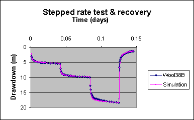
| Figure 11. Stepped test analysis |
Now the measured data, together with the type curve based on the above values, will be displayed. Your aim is to obtain the closest possible match between the two curves. (Press [F1] at any time for a help page.)
I recommend the following procedure.
Start with adjusting the coefficient 'B' by pressing [2] and then
using the up and down arrow keys. (You press [1] to adjust A, [2]
for B, [3] for C, and [4] for D).
There are two options which you should try at some stage. Pressing [d] (lower case) will decrease the range of the graph and spread the recovery data over a wide area of the VDU screen. Go in the other direction by pressing [i]. (If you get lost, press [F1]; on exit from the help screen the graph will be refreshed.) Pressing [c] will allow you to change the magnitude of the adjustment that is made whenever you press the up or down arrows.
After you have obtained the best possible fit for B, adjust A (select by pressing [1]) until you have a fair fit for the first drawdown stage. Now adjust C until you have a reasonable fit for the third drawdown stage. You will need to alternate between these two steps until you obtain a good fit overall, but you will not find it difficult.
Press [F1] to check the values of all the coefficients. When you have obtained a good fit you should find values similar to: A=0.0116, B=0.0015, C=3.1e-6, and D=2. Transmissivity will be about 124 m2/day.
You will find that it is impossible to simultaneously obtain a good fit for all three drawdown stages so long as D=2. After having done the best you can you should adjust C and D until no further improvement can be obtained. (Some modification of A will also be required. You will also find it very helpful to modify the size of the adjustments by pressing [C].) This should get you to something like: A=0.0129, B=0.0015, C=1e-10, and D=3.4.
|
Home Top Index |
Call the Well Equation option from the primary menu and you will see that the values you finished with in CGPAnal are loaded into the well equation. You will be informed that for Q=1293 m3/day and t=0.125 days (the discharge rate and finishing time for the third drawdown step) the calculated drawdown is 18.61 m. (This is slightly different to the drawdown at the end of the third step because this latter calculation is for a constant rate rather than for three steps.)
You will now be able to very quickly calculate that, given this particular well equation, a discharge rate of 1000 m3/day for a duration of 1 day will give 14.44 m drawdown, while 1000 m3/day for one year will give 18.28 m drawdown.
Example file WOOL38C has been produced from WOOL38B and simply by deleting everything after the first stage. Call aquifer test analysis (CGAnal) from the primary menu, load file WOOL38C, request a semilogarithmic graph, and select Transmissivity.
As described above, this method calculates T from a line of best fit through the 'straight line' section of the drawdown curve. The data of this stage has not settled down to a straight line, this is probably mainly due to well storage effects. We will avoid the worst affected part of the data by using the later part of the stage.
Move the first marker along to the right hand end of the data and press [Enter] to anchor it. Then move the second marker to 0.01111 days and press [Enter] again. The line of best fit will now be calculated from the selected data and transmissivity will be calculated from that. You should obtain T approximately equal to 114 m2/day.
The 114 obtained from drawdown here is close to the 124 obtained from recovery in Tutorial G8, but you will find that in many cases the difference is larger, although apparently always in the same direction.
The units must again be the set based on metres and days as the simulation is going to be based on an analysis in those units.
First we must obtain the information that we need for the analysis. We have the values for the coefficients of the well equation from Tutorial G7: A=0.0129, B=0.0015, C=1e-10, and D=3.4. The remainder can be obtained from a look at the WOOL38B data file as that is the data on which the analysis was done.
From the primary menu, check that the data subdirectory is still CGXAMPLE (Change configuration), then call CGEdit (Data entry and editing) and load file WOOL38B. Make a note of the two figures for R(aq.) and R(w.l) displayed on the main menu page of CGEdit, both of these are 0.148 m.
|
Home Top Index |
Now select Data entry/editing and then use the [PgDn] key to find the discharge rate and finishing time for each step, don't forget that the recovery period is considered to be another step (the forth in this case). The finishing time and corresponding discharge rate will be found to be as below:
| Step | Finish (days) | Discharge rate (m3/day) |
| Step 1 | 0.04167 | 485 m3/day |
| Step 2 | 0.08333 | 816 |
| Step 3 | 0.125 | 1293 |
| Step 4 | 0.146 | 0 |
This is all that is needed for the simulation, so return to the primary menu by pressing [F10] and [A].
Call program CGPDD (by selecting Well test simulation). Request an isotropic aquifer simulation (press [I]), confined (press [Y]es). Type in the above values for A, B, C, and D, as requested. Answer that there are 4 pumping steps and give the times and discharge rates as above. Reply with 0.148 for the two radius questions, and reply in the affirmative when asked whether well storage should be considered.
A series of time/drawdown/discharge test values will now be calculated and displayed. Some explanation of these is worthwhile.
Finally, view a graph of both files TEMP and WOOL38B by using program CGPlot as explained in the last part of Tutorial G3, with the difference that a linear graph might be better for these data.
From the primary menu select Change configuration, then change all the units until you have a consistent set based on feet and seconds. (At this stage the program will confirm that your units are consistent.)
Now follow the steps as above until it is time to enter the first approximations for the coefficients. This time you might enter A=20, B=10, C=50, and D=2. On adjustment of A, B, and C, you should find that the best fit is about A=35, B=12, and C=66 (assuming D is left at 2). Transmissivity will be about 0.016 ft2/sec.
This tutorial could be followed by a similar exercise to that of Tutorial G8.
The example file is an extreme case of data not generally considered amenable to analysis for aquifer values, it consists of drawdowns (and some recoveries) recorded in a piezometer during a step test. Even worse, the first stage and a part of the second stage was missed because the contractor started earlier than I was expecting.
|
Home Top Index |
|
| Figure 12. Aquifer test analysis on step test data |
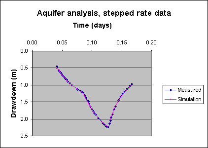
Select subdirectory CGXAMPLE, call CGAnal (Aquifer test analysis) from the primary menu and load file WAFFLB. Request a linear graph, the Automatic Generalised solution, a confined aquifer, and no boundaries. Reply that no values are known (this feature allows you to enter one value that you might feel you know in some cases, say transmissivity, and have the others evaluated by the computer) and request 20 pointers (the more pointers the slower the solution).
Now, as in Tutorial G2, you mark the data that you are interested in. First, move the single marker to the right side of the screen, using the right arrow key; then press [Enter]. Now you can accept all the provisional pointers, one by one, except for the one on the left side, at 60 minutes. This was not a measured drawdown, but is required to mark the beginning of the second drawdown step. Move this pointer to some other part of the graph.
When you have fixed the location of the last pointer you will be requested to enter your initial guesses for transmissivity and storage coefficient. Try 50 and 0.0003.
The solution will now run for a short time, depending on the speed of your computer and should then report final values of about T=100 and S=0.00044. On pressing a key the calculated points will be shown against your selected points and the other data points.
Next select the Manual Generalised solution, confined aquifer, no boundaries, and enter T=100 and S=0.00044 (or similar). You can then experiment with modifying these values and watch the effect on the type curve.
Further experiments could be carried out on file WAWIBOC which contains data from a pumped well, and WABBLB which contains data collected from a piezometer during an aquifer test.
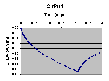
Data file CLRPU1 contains time-drawdown data from a piezometer in an area of steeply dipping and deeply weathered hard rock. This piezometer was 72.6 metres from a well which pumped at a steady rate of 562 cubic metres per day for a period of 0.21181 days (5 hours, 5 minutes). Files CLRPU1S1 and CLRPU1S2 contain simulations based on two analyses if the data of CLRPU1.
Set the units to the metre-day consistent set and make the current data file subdirectory CGXAMPLE using option 'Change Configuration' from the primary menu.
As the first step it would be advisable to examine file CLRPU1 on several graphs to confirm that we are dealing with data from a strip aquifer. Call the graphing program, CGPlot, from the primary menu, load file CLRPU1 and plot it on a semilogarithmic graph on screen, leave the recovery data unchanged. There are two things to note on this graph: the data shows a continuous downward curve to the end of discharge, and there is no straight line section before the commencement of the downward curve. This very early onset of strip aquifer behaviour indicates that the width of the strip must be similar to, or smaller than, the distance from the piezometer to the pumped well. Ignore the plotted recovery data for the present.
|
Home Top Index |
Now plot the same data on a square root of time graph. This time note that the plots fall along something close to a straight line, again indicative of a strip aquifer. Replot the file on a square root of time graph, but this time with the recovery data plotted as the square of root t minus root t'. You will observe that the recovery data now also fall close to a straight line, more evidence of a strip aquifer.
For the analysis call the aquifer analysis program from the primary menu and load the data file CLRPU1. When asked how to treat recovery data reply [N] for 'No change'. Request a semilogarithmic graph.
From the aquifer test analysis menu select Transmissivity and highlight the first five points, 0.00091 to 0.00903 days. The program calculates the Delta s slope of the best fit line through these points and then determines the transmissivity value from that, the result should be 4396 m2/day. (The transmissivity value will be highly dependent on the data chosen for calculation because of the downward curve, for example, using the first four points, 0.00091 to 0.00694 days would yield a transmissivity of 4898.)
Storage should be calculated next, select it from the menu. Transmissivity was calculated for the early time data so storage should be calculated for data in this vicinity too. Select the point corresponding to t=0.00903 days, give the T value calculated above, 4396, and storage should be calculated as 0.00137.
We now have first approximations of T and S, so we can move on to obtaining a figure for the width of the strip. Pick 'Automatic generalised' from the menu, define the aquifer type as Confined and Strip, reply that no values are known and request 15 pointers. Place the first pointer right over at the end of recovery, press [Enter] and then accept all the provisional pointer positions by pressing [Enter] another fifteen times (or hold the key down for a short time). Give the T and S values already obtained, and as your guess for strip aquifer width give 73m (about the distance from the piezometer to the pumped well). The program will now cogitate for some time and should produce parameter values of T=3967, S=0.00237, strip width=255, and a root-mean-square error value of 0.00267. (A model based on these values was used to produce simulation CLRPU1S1.)
Note here that different results will be obtained if you give different first guesses or you mark different points, eg. an alternative result is T=1160, S=0.00393, strip width=365, giving an rms error of 0.00244 (this model was used to produce example data file CLRPU1S2). It also should be mentioned that the drawdown curve for strip aquifer data is somewhat dependent on the location of both the pumped well and the piezometer within the strip. For simplicity, however, this analysis assumes that both wells are in the centre of the strip.
Finally, it is worth running the 'Manual generalised' solution to view the quality of the fit. Try it with both the above sets of values, one at a time. Press [F1] and check the root-mean-square error, this will differ from the rms error that resulted from the automatic fit because that used only 15 data points, the manual fit uses all the data. Try plotting the measured values and the two simulations on screen at the same time too.
The data that will be entered is a subset of those which makes up data file CLRPU1.
|
Home Top Index |
| Time | Water levels | Discharge rate | Remarks |
| min;sec | metres | litres/sec. | |
| 0 | 7.001 | 0 | |
| 1;19 | 7.003 | 6.5 | Flow rate started at zero time. Water level was unchanged at 1 minute 19 secs. |
| 4;13 | 7.011 | ||
| 7 | 7.017 | ||
| 13 | 7.027 | ||
| 19 | 7.034 | ||
| 26;20 | 7.043 | ||
| 37;20 | 7.053 | ||
| 47 | 7.060 | ||
| 56 | 7.067 | ||
| 72 | 7.076 | ||
| 86 | 7.086 | ||
| 117 | 7.102 | ||
| 162 | 7.121 | ||
| 208 | 7.138 | ||
| 265 | 7.158 | ||
| 300 | 7.170 | ||
| 305 | The pump was switched off. | ||
| 305.7 | 7.171 | 0 | First recovery reading. |
| 306.5 | 7.170 | ||
| 307;20 | 7.168 | Water level responding to end of discharge. | |
| 308;26 | 7.166 | ||
| 310 | 7.163 | ||
| 314 | 7.157 | ||
| 320 | 7.150 | ||
| 330 | 7.141 | ||
| 342 | 7.133 | ||
| 358 | 7.122 | ||
| 390 | 7.107 | ||
| 420 | 7.097 | Last recovery reading |
Note that the times in the list are a mixture of whole minutes, decimal minutes, and minutes and seconds (with a semicolon as a divider).
Call 'Data entry and editing' (CGEdit) from the primary menu and reply that you do not wish to load a data file.
From the CGEdit menu call 'Data entry/editing'. Reply that the data is from a piezometer, not a pumped well. The distance from the pumped well is 72.6 metres and the diameter of the well in the water level area may be entered as 0.075 metres.
After this entry you will be in the main data entry area, and in 'Add to end' mode (ie. the program will be expecting you to add data to the end of the incipient file).
Enter the first time as 0, the first 'drawdown' as 7.001, and the first discharge rate as 0. As the second record, enter time as '1;19' (meaning 1 minute and 19 seconds, most characters will serve as the divider if you would prefer something other than a semicolon) and drawdown as 7.003. You will find that you are not asked for a discharge rate, it will be copied from the previous record. The reason for this will become clear later. You will also notice that the time entry has been converted to decimal minutes.
|
Home Top Index |
|
| Figure 13. The full data set |
Type in the remaining recovery values, press [Esc] to get back to 'Data entry/editing' and [F10] to go to the CGEdit main menu.
If you have made any typographic errors they will probably be fairly obvious. Make a note of them, go back to CGEdit and correct them. Figure 13 shows the whole of the data file (CLRPU1), your data should look similar.
Exit back to the main menu, press [5], and save the data. Use the same file name, CLRPU1B.
From the primary menu select Change configuration and then change the time unit to days and the discharge rate unit to cubic metres per day. You are now ready for analysis.
|
Home Top Index |
Clarke, D.K., 1988. Groundwater Discharge Tests: Simulation and Analysis. Elsevier Sci. Pub., Sara Burgerhartstraat 25, P.O. Box 211, 1000 AE Amsterdam, The Netherlands.
Cobb, P.M., Mc Elwee, C.D., and Butt, M.A., 1982. An Automated Numerical Evaluation of Leaky Aquifer Pumping Test Data: An Application of Sensitivity Analysis. Kansas Geo. Survey.
Hantush, M.S., and Jacob, C.E., 1955. Non-steady radial flow in an infinite leaky aquifer: Transactions of the American Geophysical Union, v. 36, pp. 95-100.
Kruseman G.P. and DeRidder N.A., 1983. Analysis and evaluation of Pumping Test Data. Bulletin 11, Internal Inst. for Land Reclamation and Improvement, Wageningen, The Netherlands.
McElwee, C.D., 1980. The Theis equation: evaluation, sensitivity to storage and transmissivity, and automated fit of pump test data. Kansas Geol. Syv., Uni. of Kansas, Lawrence, Kansas 66044, U.S.A.
Muskat, M., 1937. The Flow of Homogeneous Fluids through Porous Media. McGraw Hill Book Co., New York.
Theis, C.V., 1935. The relation between the lowering of the piezometric surface and the rate and duration of discharge of a well using groundwater storage. Trans. Am. Geophs. Un. 16:pp519-524.